A Closer Look at the k-Nearest Neighbors Algorithm
As far as machine learning algorithms go, the k-nearest neighbors algorithm is one of the simplest to understand. If you examine the algorithm a little more closely, though, you’ll notice it’s more nuanced than is readily apparent. This week I had a chance to read up on similarity-based learning in Fundamentals of Machine Learning for Predictive Data Analytics. There are a couple topics they cover that I thought were of note and shed some light on the multiple ways in which the KNN algorithm can be implemented and difficulties around its implementation. Specifically, I’ll be discussing cosine similarity and k-dimensional binary trees.
So, to start with, let’s describe the k-nearest neighbors algorithm. You have a sample and you want to predict the value of one of its features. We’ll refer to this sample as the query sample and the feature in question as the query feature.
Following the steps of the KNN algorithm, each sample in the training dataset is compared to the query sample. The values of the query feature for each of the k most similar training samples is tallied up. If the domain of the query feature is continuous (e.g. any real number between one and ten), then the average of the k samples is the predicted value on the query sample for the query feature. If the domain is made up of discrete values (e.g. ‘yes’, ‘no’, ‘up’, ‘down’), then the feature value that appears most often in the k samples is the predicted value for the query feature.
Cosine Similarity
The Minkowski distance is often used to measure the similarity between a training sample and the query sample.

The most common measure of similarity is the Minkowski distance where p = 2. You’ll recognize this as the Euclidean distance:

An alternative measure of similarity is cosine similarity. Cosine similarity is measured by taking the cosine of the angle between the two vectors in the feature space that represent the query and training samples. Each vector starts at the origin.
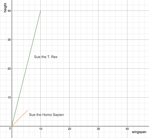
2-d feature space
You may recall from linear algebra that the equation for the dot product of two vectors  and
and  is
is

There is a relationship between the dot product of two vectors and the angle θ between them:

Hence, we can measure the cosine similarity of training sample p and query sample q like so:

If the cosine of the angle between  and
and  is one, then the two vectors have the same slope, i.e. the ratio of the relevant features is the same for each of them. Cosine similarity is used in situations where the absolute magnitude of a feature isn’t important, just its value relative to another feature.
Dealing with Large Training Sets
The k-nearest neighbor algorithm can easily become computationally expensive. For every query sample, you need to iterate through the entire training set and calculate the similarity between each training sample and the query sample.
One way to mitigate that is to use a k-dimensional binary tree (often called a ‘k-d tree’ for short). Each node of the k-d tree is a sample from the training set. The k refers to the dimension of the feature space occupied by the samples.
Let’s consider a concrete example. We would like to be able to guess if a person is a machine learning engineer based on how many times they use the words “Westworld” or “Python” in conversation in a week.
| ID | python refs | westworld refs | MLE? |
|---|---|---|---|
| A | 3 | 8 | no |
| B | 10 | 7 | no |
| C | 12 | 11 | yes |
| D | 8 | 15 | yes |
| E | 14 | 3 | yes |
| F | 12 | 17 | yes |
| G | 9 | 14 | no |
| H | 3 | 1 | no |
| I | 13 | 19 | yes |
| J | 18 | 19 | yes |
| K | 11 | 6 | no |
| L | 7 | 2 | no |
| M | 15 | 5 | yes |
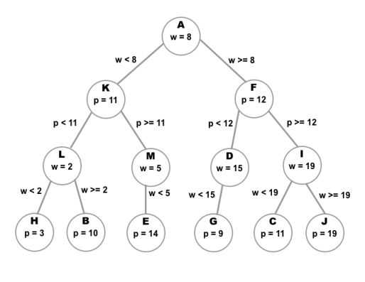
To construct the tree, we choose one of the features, say, Westworld references (w), and find the training sample that has the median value for that feature. We then store that sample in the root node.
Next, we need to find values for the left and right child nodes. The left child and all of the nodes in its subtree will have values for w that are less than the median value. Every node from the right child down will have values greater than or equal to the median.
Of course, there will (hopefully) be more than just three samples to work with. We’ll need to split both the samples on the left and the right in the same way that we did for the first node. This time, however, we will use the number of Python references (p) the person has made.
We repeat this process, alternating between each feature for each level of the tree and splitting the set of remaining samples by its median value, until we are out of samples.
The result is a tree that can be represented like so
To simplify things, we will look for the single closest sample to our query sample. We start at the root node and step down each node according to the feature values of the query sample. So, for instance, if the query sample has a value for w that is greater than or equal to the w value of the root node, we step down to the right child node. At the next level, we compare the query sample’s p value to the p value of the current node and go right or left accordingly. We repeat this process until we reach a leaf node. When a leaf node is reached, we designate it as the nearest node.
We then climb back up the tree. Here’s where the k-d tree is really useful. Again, we have a node that we have designated as the nearest node. For this example, let’s say we’re using Euclidean distance as the similarity metric. That means we are asserting that the Euclidean distance dn between the query and the nearest node is smaller than the distance between the query and any other node.
dn is the radius of a circle enclosing the query sample. For another node to be the nearest, it must lie within the borders of that circle. That means it cannot be further than dn along the w axis or the p axis.
As we are stepping from node to node up the tree, we will have to decide at each node if we want to check the subtree starting at the current node’s other child or if we want to move up to the current node’s parent. The current node holds the median value used to divide the samples into two groups. Essentially, it sits between the values on its left branch and the values on its right for some splitting feature. Thus, all we need to do is check the difference between the splitting feature for the current node and the splitting feature for the query sample against dn. If the splitting feature difference is greater than dn, we move up to the parent of the current node. Otherwise, we must traverse down the other branch to search for nodes even closer than nearest.